6. Basis sets
6.1. LAPW basis
The reader is supposed to be familiar with the LAPW basis set. This section is intended as a short recapitulation and to define the notation used in the manual.
The LAPW method relies on a partitioning of space into non-overlapping MT spheres centered at the atomic nuclei and the interstitial region. The basis functions are defined differently in the two regions, plane waves in the interstitial and numerical functions in the spheres, consisting of a radial part \({u_{lp}^a(r)}\) (\({a}\) is the atomic index) and the spherical harmonics \({Y_{lm}(\hat{\mathbf{r}})}\). \({p}\) is an index to distinguish different types of radial functions: \({u_{l0}^a=u_l^a}\), \({\,u_{l1}^a=\dot{u}_l^a=\partial u_l^a/\partial\epsilon}\), \({\,u_{lp}^a=u_l^{a,\mathrm{LO}},\,p\ge 2}\), where we have used the usual notation of LAPW. Augmented plane waves are formed by matching linear combinations of the \({u}\) and \({\dot{u}}\) to the interstitial plane waves, forming the standard LAPW basis set. Local orbitals \({u^\mathrm{LO}}\) can be used to extend the basis set, to enable the description of semicore and high-lying conduction states. The plane waves and the angular part of the MT functions can be converged straightforwardly with the reciprocal cutoff radius \({g_\mathrm{max}}\) and the maximal l quantum number \({l_\mathrm{max}}\), respectively, whereas the radial part of the MT functions is more difficult to improve systematically, but it is possible, see [Comput. Phys. Commun. 184, 2670 (2013)].
Running the one-shot mean-field calculation with Spex (using ITERATE, see Section 4.2.9) offers the possibility of
modifying the LAPW basis in “spex.inp”. This can be useful for GW calculations, which require an accurate basis for a much larger
energy range (including many unoccupied states) than in DFT.
The respective keywords are defined in the section LAPW and are described in the following.
6.1.1. GCUT (LAPW)
The set of G vectors depends on the k point and is defined with the cutoff condition \(|\mathbf{k}+\mathbf{G}|<G_\mathrm{cut}\).
The parameter \(G_\mathrm{cut}\) can be defined with the keyword GCUT, e.g., GCUT 4.0 (in Bohr-1).
6.1.2. LCUT (LAPW)
In the muffin-tin spheres, the basis functions are expanded in radial functions \(u_{lp}(r)\) and spherical harmonics
\(Y_{lm}(\hat{\mathbf{r}})\).
The keyword LCUT lets you define the cutoff for the l quantum number separately for each atom type.
LCUT 10 8 |
An l cutoff of 10 and 8 is used for the first and second atom type, respectively. |
6.1.3. EPAR (LAPW)
The radial functions \(u_{lp}(r)\) are determined from scalar-relativistic Dirac equations inside the MT spheres with energy
parameters \(E_{lp}\). (As one cannot impose a boundary condition at the MT boundary, the energy does not result
from the solution as an eigenvalue but must be provided as a parameter.)
The energy parameters for the functions \(u_{l0}(r)\) [usually denoted by \(u_l(r)\)] and \(u_{l1}(r)\)
[\(\dot{u}_l(r)\)] (having the same parameter in a given l channel) are defined with the keyword EPAR.
There can be at most as many arguments as atom types.
(For atom types without an explicit definition, the energy parameters remain unchanged.)
Each argument is bounded by parentheses (...). An empty definition () is allowed and means that the energy parameters of this
atom type remain unchanged. Otherwise, one writes a comma-separated list of parameters starting at \(l=0\) (then, \(l=1\), etc.).
Parameters not given will just be set identical to the last one given. A wildcard (*) selects the energy parameter from the
input data. Energy parameters can be given explicitly as real numbers (in Hartree or eV with the unit eV) or as main quantum numbers of the atomic shell.
The usage is shown in the examples.
EPAR (-0.01,0.04,0.06) |
The energy parameters for s, p, d, and f (etc.) functions are defined to be -0.01, 0.04, 0.06, 0.06 (etc.). (All values in Hartree.) |
EPAR () (-0.01/-0.005,*,3,*) |
The energy parameters for the first atom type are unchanged. The energy parameters for the s functions of the second atom type are -0.01 htr for spin up and -0.005 htr for spin down. The parameters for the p functions are unchanged from the input. The parameters for the d functions are taken from an atomic solver (3d orbital) for both spins. The parameters for higher l are unchanged. |
EPAR () (-0.01/-0.005,*,3d,*) |
Same as before. The possibility of defining 3d explicitly is included for better readability of the input file. |
6.1.4. LO (LAPW)
Local orbitals (LOs) are used to improve the basis set in the atomic MT spheres. There are two use cases: First, to describe low-lying
semicore states (which are too close to the valence bands to be described as core states confined in the MT spheres).
Second, to improve the description of high-lying unoccupied states, which are relevant for GW calculations and, generally, for
response quantities. LOs are defined by a similar syntax as EPAR. However, there is no fixed order in the l quantum number.
Therefore, one
always has to define the l quantum number together with the energy parameter or the main quantum number. Since there is no
fixed order, the wildcard (*) used in EPAR to “skip” l quantum numbers is unnecessary and not available.
However, there is another use of the
wildcard (*). If given as the first argument (without parentheses), the LOs from the input data are kept and the new LOs
are added to this set. Without *, only the LOs defined after LO will be used (and the ones from the input data are
removed). There is a special LO definition that lets Spex automatically add local orbitals to improve the MT basis representation
for unoccupied states. In particular, Spex adds local orbitals in such a way that the MT basis is able to accurately represent
states over the energy range \(v_0<\epsilon<v_0+G_\mathrm{cut}^2/2\) with the average effective potential \(v_0\) and
the momentum cutoff \(G_\mathrm{cut}\). [In this energy range, the wavefunctions are well described in the interstitial
region (by the plane-wave basis defined with \(G_\mathrm{cut}\).)]
Here, “accurate” means that states in this energy range can be represented in the MT spheres within an accuracy of at least 99%
(also see keyword MTACCUR, Section 4.2.12).
An example for this special LO definition is spd:+, in which case
LOs would be automatically added in the s, p, and d channel.
Note that adding many local orbitals can make the basis set so flexible that core states might appear as eigenstates
(perhaps badly described as high-lying “ghost” bands). In this case (if the spurious band is below and well separated
from the valence region), ITERATE allows the specification of an eigenenergy cutoff below which all eigenstates are
cut away.
The usage of the keyword LO is shown in the examples.
LO (s:-30.4eV,p:-29.2eV) |
Define s and p local orbitals with explicit energy parameters -30.4 and -29.2 eV.
(The default unit, i.e., without eV, is Hartree units.) |
LO (l=0:-30.4eV,l=1:-29.2eV) |
Same as before defined with an alternative syntax. |
LO (l=0:-30.4eV/-29.5eV,l=1:-29.2eV/-28.3eV) |
Same as before for a spin-polarized system. |
LO () (3s,3p) |
Define s and p local orbitals for the second atom type with parameters obtained from an atomic solver (for the description of semicore states). |
LO (3d,spd:+) |
Define 3d local orbital and let Spex automatically add local orbitals to improve the description of the unoccupied spectrum in the s, p, and d channel. |
LO * (spd:+) |
Add higher-energy local orbitals as before but also keep local orbitals from the input file (which might include semicore LOs.) |
6.1.5. MTACCUR (ANALYZE)
(*) The accuracy of the radial MT basis can be analyzed with the keyword MTACCUR followed by two numbers \(e_1\) and \(e_2\).
Spex then calculates the MT representation error
[Phys. Rev. B 83, 081101] in the energy range between \(e_1\) and \(e_2\).
(If unspecified, upper and lower bounds are chosen automatically.)
The results are written to the output files “spex.mt.t” where t is the atom type index,
or “spex.mt.s.t” with the spin index s(=1 or 2) for spin-polarized calculations. The files contain sets of data for all l quantum numbers, which can be plotted separately with “gnuplot” (e.g., plot "spex.mt.1" i 3 for \({l=3}\)).
MTACCUR -1 2 |
Calculate MT representation error between -1 and 2 Hartree. |
MTACCUR |
Automatic energy range. |
6.2. Mixed product basis
The methods implemented in Spex distinguish themselves from conventional DFT with local or semilocal functionals by the fact that individual two-particle scattering processes are described explicitly. In such processes, the state of an incoming particle and the state that it scatters into form products of wavefunctions. Many of the physical quantities, such as the Coulomb interaction, the polarization function, and the dielectric function, become matrices when represented in a suitable product basis. In the context of the FLAPW method, the mixed product basis is an optimal choice. It consists of two separate sets of functions that are defined only in one of the spatial regions, while being zero in the other, the first is defined by products of the LAPW MT functions and the second by interstitial plane waves. (The products of plane waves are plane waves again.) The corresponding parameters are defined in the section MBASIS of the input file.
6.2.1. GCUT (MBASIS)
If \({N}\) is the number of LAPW basis functions, one would naively expect the number of product functions to be roughly \({N^2}\). In the case of the interstitial plane waves, this is not so, since, with a cutoff \({g_\mathrm{max}}\), the maximum momentum of the product would be \({2g_\mathrm{max}}\), leading to \({8N}\) as the number of product plane waves. Fortunately, it turns out that the basis size can be much smaller in practice. Therefore, we introduce a reciprocal cutoff radius \({G_\mathrm{max}}\) for the interstitial plane waves and find that, instead of \({G_\mathrm{max}=2g_\mathrm{max}}\), good convergence is achieved already with \({G_\mathrm{max}=0.75g_\mathrm{max}}\), the default value. The parameter \({G_\mathrm{max}}\) can be set to a different value with the keyword GCUT in the section MBASIS of the input file.
GCUT 2.9 |
Use a reciprocal cutoff radius of 2.9 Bohr-1 for the product plane waves. |
6.2.2. LCUT (MBASIS)
The MT functions are constructed from the products \({u_{lp}^a(r)Y_{lm}(\hat{\mathbf{r}})u_{l'p'}^a(r)Y_{l'm'}(\hat{\mathbf{r}})}\). (Obviously, the atom index \({a}\) must be identical.) The product of spherical harmonics expands into a linear combination of \({Y_{LM}(\hat{\mathbf{r}})}\) with \({L=|l-l'|,...,l+l'}\) and \({|M|\le L}\). In principle, this leads to a cutoff of \({2l_\mathrm{max}}\) for the products, but, as with the plane waves, one can afford to use a much smaller cutoff parameter in practice. We use \({L_\mathrm{max}=l_\mathrm{max}/2}\) as the default. The corresponding keyword in the input file is called LCUT.
LCUT 5 4 |
Use l cutoffs of 5 and 4 for two atom types in the system. |
6.2.3. SELECT (MBASIS)
In the LAPW basis, the matching conditions at the MT boundaries require large l cutoff values, typically around \({l=10}\), giving a correspondingly large number of radial functions. Not all of these functions must be considered in the product basis set. The keyword SELECT enables a specific choice of the radial functions. When specified, an entry for each atom type is required.
The best way to describe the syntax of SELECT is with examples:
SELECT 2;3 |
Use products of \({u_{lp} u_{l'p'}}\) with \({l\le 2}\) and \({l'\le 3}\) for \({p=0}\) (so-called \({u}\)) and no function of \({p=1}\) (so-called \({\dot{u}}\)). |
SELECT 2,1;3,2 |
Same as before but also include the \({\dot{u}}\) functions with \({l\le 1}\) and \({l'\le 2}\). |
SELECT 2,,1100;3,,1111 |
Same as first line but also include the local orbitals \({p\ge 2}\), which are selected (deselected) by “1” (“0”): here, the first two and all four LOs, respectively. The default behavior is to include semicore LOs but to exclude the ones at higher energies. |
SELECT 2,1,1100;3,2,1111 |
Same as second line with the LOs. |
The LOs are selected by series of 1s and 0s. If there are many LOs, a definition like 0000111
can be abbreviated by 4031 (four times 0, three times 1).
One of the most important quantities to be calculated in GW calculations (and related methods)
are the “projections”
\({\langle M_{\mathbf{k}\mu} \phi_{\mathbf{q}n} | \phi_{\mathbf{k+q}n'} \rangle}\),
which describe the coupling of a propagating particle to an interaction line. Often, the two states with
\(n\) and \(n'\) are occupied and unoccupied, respectively.
In this sense, the first set of SELECT parameters before the semicolon refers to the occupied states,
the set after the semicolon refers to the unoccupied states.
For \(l=2\) with \(2l\) or \(2l+1\) being the l cutoff specified by LCUT, the default
would be 2;3.
6.2.4. TOL (MBASIS)
(*) The set of MT products selected by SELECT can still be highly linearly dependent. Therefore, in a subsequent optimization step one diagonalizes the MT overlap matrix and retains only those eigenfunctions whose eigenvalues exceed a predefined tolerance value. This tolerance is 0.0001 by default and can be changed with the keyword TOL in the input file.
TOL 0.00001 |
Remove linear dependencies that fall below a tolerance of 0.00001 (see text). |
6.2.5. OPTIMIZE (MBASIS)
Despite the favorable convergence behavior of the mixed product basis,
it can still be quite large. In the calculation of the screened interaction, each matrix element, when represented in the basis of Coulomb eigenfunctions, is multiplied by \({\sqrt{v_\mu v_\nu}}\) with the Coulomb eigenvalues \({\{v_\mu\}}\). This gives an opportunity for reducing the basis-set size further by introducing a Coulomb eigenvalue threshold \({v_\mathrm{min}}\). The reduced basis set is then used for the polarization function, the dielectric function, and the screened interaction. The parameter \({v_\mathrm{min}}\) can be specified after the keyword OPTIMIZE MB in three ways: first, as a “pseudo” reciprocal cutoff radius \({\sqrt{4\pi/v_\mathrm{min}}}\) (which derives from the plane-wave Coulomb eigenvalues \({v_\mathbf{G}=4\pi/G^2}\)), second, directly as the parameter \({v_\mathrm{min}}\) by using a negative real number, and, finally, as the number of basis functions that should be retained when given as an integer. The so-defined basis functions are mathematically close to plane waves. For testing purposes, one can also enforce the usage of plane waves (or rather projections onto plane waves) with the keyword OPTIMIZE PW, in which case the Coulomb matrix is known analytically. No optimization of the basis is applied, if OPTIMIZE is omitted.
OPTIMIZE MB 4.0 |
Optimize the mixed product basis by removing eigenfunctions with eigenvalues below \(4\pi/4.0^2\). |
OPTIMIZE MB -0.05 |
Optimize the mixed product basis by removing eigenfunctions with eigenvalues below 0.05. |
OPTIMIZE MB 80 |
Retain only the eigenfunctions with the 80 largest eigenvalues. |
OPTIMIZE PW 4.5 |
Use projected plane waves with the cutoff 4.5 Bohr-1 (for testing only, can be quite slow). |
In summary, there are a number of parameters that influence the accuracy of the basis set. Whenever a new physical system is investigated, it is recommendable to converge the basis set for that system. The parameters to consider in this respect are GCUT, LCUT, SELECT, and OPTIMIZE.
Finally, we show a section MBASIS for a system with three atom types as an example
SECTION MBASIS
  GCUT 3.0
  LCUT 5 4 4
  SELECT 3,2;4;2 2;3 2;3
  TOL 0.0001
  OPTIMIZE MB 4.5
END
6.2.6. NOAPW (MBASIS)
(*) By default, Spex constructs augmented plane waves from the mixed product basis in a similar way as in the LAPW approach. In this way, the unphysical “step” at the MT sphere boundaries is avoided. It also leads to a further reduction of the basis set without compromising accuracy. This APW construction can be avoided with the keyword NOAPW.
6.2.7. ADDBAS (MBASIS)
(*) This keyword augments the mixed product basis by the radial \({u_{lp}}\) functions, the \({l}\) and \({p}\) parameters are according to the first part of the SELECT definition. This improves the basis convergence for COHSEX calculations.
6.2.8. CHKPROD (MBASIS)
(*) Checks the accuracy of the MT product basis.
6.2.9. WFADJUST (MBASIS)
(**) Removes wavefunction coefficients belonging to radial functions that are not used to construct the MT product basis. (Currently the coefficients are actually not removed from memory.)
6.2.10. FFT (WFPROD)
(*) When the interaction potential is represented in the mixed product basis, the coupling to the single-particle states involve projections of the form
\({\langle M_{\mathbf{k}\mu} \phi_{\mathbf{q}n} | \phi_{\mathbf{k+q}n'} \rangle\,.}\)
The calculation of these projections can be quite expensive. Therefore, there are a number of keywords that can be used for acceleration.
Most of them are, by now, somewhat obsolete. An important keyword, though, is FFT in the section WFPROD of the input file.
When used (see examples), the interstitial terms are evaluated using Fast Fourier Transformations (FFTs), i.e.,
by transforming into real space (where the convolutions turn into products), instead of by explicit convolutions in reciprocal space.
For small systems the latter is faster, but for large systems the FFTs give a better scaling with system size (see note).
The optional argument gives the reciprocal cutoff radius used for the FFT.
A run with FFTs can be made to yield results identical to the explicit summation. This requires an FFT reciprocal cutoff radius of at least
\({2g_\mathrm{max}+G_\mathrm{max}}\), which can be achieved by setting FFT EXACT, but such a calculation is quite costly. It is, therefore, advisable to use smaller cutoff radii, thereby sacrificing a bit of accuracy but speeding up the computations a lot. If given without an argument, Spex will use 2/3 of the above exact cutoff,
which is a compromise between precision and computational cost.
One can also specify an explicit cutoff by a real-valued argument explicitly.
Typical values are between 6 and 8 Bohr-1.
Note
(Since version 05.06:) FFTs are included by default for large systems (unit-cell volume larger than 1200 Bohr3) with the reciprocal cutoff radius \({\frac{2}{3}(2g_\mathrm{max}+G_\mathrm{max})}\). Otherwise, explicit convolutions are used.
FFT 6 |
Use FFTs with the cutoff 6 Bohr-1. |
FFT |
Use the default cutoff \({\frac{2}{3}(2g_\mathrm{max}+G_\mathrm{max})}\). This is the cutoff automatically used for large systems. |
FFT EXACT |
Use the exact cutoff \({2g_\mathrm{max}+G_\mathrm{max}}\). |
FFT OFF |
Do not use FFTs. |
6.2.11. APPROXPW (WFPROD)
(**) Since version 02.03 the interstitial part of the projections is calculated exactly, leading to favorable convergence with respect to GCUT. However, the exact evaluation takes considerably more time. If APPROXPW is set, the old and approximate way of calculating the products is used instead. (Only included for testing.)
6.2.12. LCUT (WFPROD)
(**) The MT part of the projections can be accelerated as well using the the keyword LCUT
in the section WFPROD. This keyword should not be confused with the keyword of the same name
in the section MBASIS, Section 6.2.2. It can be used to restrict the l cutoff of the wavefunctions
(only for the projections), one l cutoff for each atom type.
6.2.13. MINCPW (WFPROD)
(**) The keyword MINCPW modifies the plane-wave wave-function coefficients such that their absolute values become as small as possible. This reduces the error in the evaluation of the wave-function products arising from the finite G cutoff and leads to better convergence with respect to GCUT and smoother band structures, when APPROXPW is used. The coefficients can be modified, because the set of IPWs is overcomplete. If set, the eigenvectors of the overlap matrix with the n smallest eigenvalues are used for this modification. Note that it only makes sense to use this together with APPROXPW.
6.3. Wannier orbitals
For many features of the Spex code, Wannier functions are required: Wannier interpolation, spin-wave calculations, GT self-energy, Hubbard U parameter. Wannier functions are constructed by a linear combination of single-particle states. They can be viewed as Fourier transforms of the Bloch states. While Bloch states have a definite k vector and are delocalized over real space, the Wannier functions are localized at specific atomic sites and delocalized in k space. The mathematical definition is
with the lattice vector \(\mathbf{R}\), the orbital index \(n\), the number of k vectors \(N\), and the transformation matrix \(U\). The Wannier orbital is localized in the unit cell at \(\mathbf{R}\) and, in most cases, at a specific atom in that unit cell. The Wannier transformation matrix \(U\) is unitary if there are as many Wannier orbitals as there are Bloch bands included in the construction. There can be more Bloch bands but not less. There are several ways to determine \(U\). The simplest is a projection method, in which the Bloch eigenstates are projected onto a localized atomic (muffin-tin) function \(u_n(\mathbf{r})\), which can be of any orbital character (including hybrid orbitals). This gives an auxiliary matrix
which is then (Loewdin) orthonormalized to yield the transformation matrix \(U\). We call the Wannier functions calculated with this \(U\) “first-guess” Wannier functions, as they can be used as the input (first-guess) functions for a disentanglement and/or maximal localization procedure with the Wannier90 library, which then yields a new, refined \(U\).
Wannier functions are defined in the section WANNIER:
SECTION WANNIER
  ORBITALS 1 4 [sp3]
  MAXIMIZE
END
The example shows the definition of four (bonding) sp3 hybrid orbitals for silicon.
6.3.1. ORBITALS (WANNIER)
This line is the main definition of Wannier orbitals giving the orbital characters for the first-guess orbitals and
the energy window. The energy window is defined by the first two arguments, the indices of the lower and upper band
[summation index \(m\) in Eq. (1)].
Note that if, in the above example, the fourth state is degenerate with the fifth at some k point, the fifth state will
automatically be included as well.
(This is the default behavior. It can be changed to excluding the fourth band or to ignoring
degeneracies altogether by setting preprocessor macros, see the source file “wannier.f”.)
A wildcard (*) can be set in place of the upper band index, which lets Spex determine a (minimal) band index
automatically. (Note that this will not necessarily yield an optimal upper index.)
After the energy window follows the
definition of the orbital characters of the projection functions used to calculate the first-guess Wannier functions.
Although strictly not guaranteed, the orbital character is usually preserved not only after projection in the
first-guess functions but even after the maximal localization
procedure (see Section 6.3.2). The orbital character is defined for each atom type (round brackets) or each atom
(square brackets). Empty brackets, such as () or [], are allowed. For example, (p) () (d)
gives three p orbitals in the first atom, five d orbitals in the third, and none in the second. The number of bands
in the energy window must not be smaller than the number of Wannier orbitals (but can be larger).
ORBITALS 1 18 [s,p,d] |
Define s, p, and d Wannier orbitals in the first (and perhaps only) atom. |
ORBITALS 6 11 (t2g) |
Define t2g Wannier orbitals in the first atom type (here two atoms) from the sixth through the 11th band. |
ORBITALS 6 * (t2g) |
Same as before, but the upper band index will be determined automatically. |
ORBITALS 1 9 [] [d] |
Define d Wannier orbitals in the second atom. |
The above example for the WANNIER section is for bulk silicon, which has two atoms in the unit cell. Four sp3 hybrid orbitals are defined
for the first and none for the second. (Trailing empty brackets as in (sp3) () can be omitted.)
In this case, the four bands of the energy window (1 4) are all formed by bonding sp3 orbitals.
Therefore, by projection, the resulting Wannier orbitals are evenly distributed over the two atoms.
This is an effect of the system’s symmetry and not explicitly caused by the particular Wannier definition.
If one wants to describe the antibonding orbitals as well, one would have to define, for example, (sp3) (sp3)
or just [sp3], and increase the energy window. Since the empty states of silicon are entangled, simply
doubling the energy window (1 8) does not suffice. We will discuss the case of entangled bands below.
The orbital characters are defined in the same way as in Wannier90. The following orbital labels are available:
s, p, d, f, g, px, py, pz, dxy, dyz, dz2, dxz, dx2y2, t2g, eg,
fz3, fxz2, fyz2, fzxy, fxyz, fxxy, fyxy, sp, sp2, sp3, sp3d, and sp3d2.
Consult the Wannier90 manual for details.
In addition, there are capitalized labels (S, P, D, F, G), in which case complex spherical harmonics are used
instead of real spherical harmonics. (Obviously, S is equivalent to s and included only for completeness.
In practice, real and complex spherical harmonics behave identically in the present context.)
Wannier functions (except for s orbitals) have an angular dependence.
Sometimes it is necessary to specify a particular spatial orientation of Wannier orbitals. For this purpose, one can
give Euler angles (in degrees), for example, (s,px/30/60/-90,d), through which the Wannier orbital (of px
symmetry in this case) is rotated; 1st angle: rotation about z axis, 2nd angle: rotation about new (rotated) x axis,
3rd angle: rotation about new (rotated) z axis.
The so-generated Wannier function are first-guess Wannier functions. As explained above, the expansion coefficients \(U_{\mathbf{k}n,m}\) are obtained from projecting the Bloch functions \(\phi_{\mathbf{k}n}\) onto localized functions with the chosen orbital character and a subsequent orthonormalization procedure to make the Wannier set orthonormal. For many purposes, the resulting set of Wannier functions is already usable. However, it is not yet maximally localized. The following keyword enforces maximal localization with Wannier90 (using the Wannier90 library), yielding the set of maximally localized Wannier functions (MLWFs).
6.3.2. MAXIMIZE (WANNIER)
The maximal localization procedure of Wannier90 is applied starting from the set of first-guess
Wannier functions. The input file for Wannier90 (“wannier.win”) is generated automatically by
Spex if it is not present yet. The user can still provide his own “wannier.win” and, in this way,
fine-tune the localization procedure. However, some of the parameters (num_wan and
num_bands) might still be changed by Spex if they are inconsistent with the Spex input
(in ORBITALS). The output of Wannier90 is written to the file “wannier.wout”. This file should
be checked for convergence of the maximal localization. For further details, consult the Wannier90
manual.
Note
MAXIMIZE requires Spex to be linked to the Wannier90 library. To this end, the Spex configure script for compilation has to be run with the option --with-wan. See Section 1.
6.3.3. FROZEN (WANNIER)
In the case of entangled bands, it is often necessary to add an extra step in the construction
of MLWFs, the disentanglement, which is also an iterative optimization procedure.
To this end, one defines a frozen energy window, which lies inside the outer energy window
defined by ORBITALS. The frozen energy window is defined by two energies, the lower and the
upper bound. By default, the lower bound is assumed to coincide with the minimum energy of the lowest band
of the outer window, i.e., the first argument of ORBITALS. If FROZEN is given without an
argument, the upper bound is guessed by Spex. This guess can be overridden by giving the upper
energy as an argument to FROZEN. Alternatively, one can specify the Wannier90 parameters
dis_froz_min and dis_froz_max in the file “wannier.win”. For illustration, the lower and upper bounds
of the frozen energy window are shown in the figure below for the example of iron (spin-up).
Giving FROZEN without MAXIMIZE
is possible. In this case, the disentanglement procedure is performed but not the maximal localization
procedure. You should check the convergence of the disentanglement procedure in the file “wannier.wout”.
For further details, consult the Wannier90 manual.
FROZEN |
Run disentanglement procedure. Frozen window bounds are guessed by Spex. |
FROZEN 5eV |
Run disentanglement procedure and use 5 eV as upper bound. |
FROZEN 8.5eV 10eV |
Run disentanglement procedure with different upper bounds for spin-up and spin-down. |
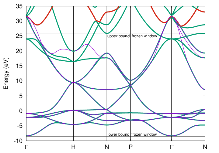
Comparison of the explicit (green lines) and Wannier-interpolated (magenta lines) DFT band structure for iron (spin-up).
The Wannier functions are constructed with ORBITALS 1 * (s,p,d), MAXIMIZE, and FROZEN.
The lower bound of the outer energy window is set at the lowest valence band (band index 1), and the upper bound
is set automatically by Spex (wildcard “*”). In this case, it is set to the 12th band, here marked in red.
The lower and upper bounds of the inner frozen energy window for disentanglement are guessed by Spex and shown
in the figure as well.
Note
FROZEN requires Spex to be linked to the Wannier90 library. To this end, the Spex configure script for compilation has to be run with the option --with-wan. See Section 1.
6.3.4. SUBSET (WANNIER)
With this keyword, a subset of Wannier functions can be selected from the full set. This can be helpful
to reduce computational cost in large systems if one is only interested in on-site parameters:
The full set (usually comprising Wannier functions at several atoms) can then be reduced to Wannier functions at a single
atom (compare Section 5.5.2). Another use case would be to select a particular shell, e.g., the d subspace, from a larger Wannier set,
e.g., (s,p,d). At first, it might be surprising that a special keyword is introduced for that, since a more intuitive way would be to
simply change the ORBITALS definition, e.g., from (s,p,d) to (d). However, the d orbitals created with a definition (d)
are different from the d orbitals created with (s,p,d). This is because the Wannier construction
(orthonormalization, disentanglement, maximal localization) is an optimization procedure that always involves the whole Wannier set.
The Wannier orbitals are not created independently of each other. So, SUBSET allows you to pick a Wannier
subset from a larger set, preserving the orbitals’ shape.
The keyword SUBSET expects a list of Wannier indices (see examples), following the order of the
generated Wannier functions. (In most cases, this order is according to the ORBITALS definition, see the
“orbital decomposition” in the output.)
SUBSET (5-9) |
Select full d shell from the set (s,p,d). |
SUBSET (1,5-7) |
Select s and t2g functions from the set (s,p,t2g). |
6.3.5. PLOT
Spex can plot the Wannier orbitals on a 3D grid and write it to XSF files for XCrySDen or Vesta
(“wannier1.xsf”, “wannier2.xsf”, etc. or “wannier1s1,xsf”, “wannier1s2.xsf”, “wannier2s1,xsf”, etc. in case of spin polarization).
The plot region and resolution can be
set with several optional arguments after PLOT: The first argument defines the units of the coordinate system: UC (unit cell), SC (supercell),
or CART (cartesian coordinates in Bohr). (The default is UC.) The second argument defines the plot region.
For example, {0:1,0:1,0:1} (this is the default) would set it to the unit cell (with UC), the supercell (with SC), or
a cube with a side length of 1 Bohr (with CART), also see figure and examples. All coordinates are with respect to the origin of the coordinate system at (0,0,0).
The resolution is set by the last three integers, giving the number of grid points
along the three dimensions. The default is “20 20 20”. (Note that 3D plots can be computationally expensive.)
PLOT |
Plot Wannier orbitals in the default plot region (unit cell) with \(20\times 20\times 20\) points. (Same as PLOT UC.) |
PLOT 30 30 30 |
Increase resolution. (Same as PLOT UC 30 30 30.) |
PLOT UC {-1:2,-1:2,0:0.5} |
Additionally, include the eight unit cells adjacent to the central one in the first two dimensions (e.g., xy plane) but cut the plot region at half the unit cell along the third dimension (e.g., z direction). |
PLOT SC {-0.5:0.5,-0.5:0.5,-0.5:0.5} |
Define the plot region to be the supercell but place the origin of the coordinate system into the center of the plot. |
PLOT CART {-1.2:2.5,-2.4:2.5,0:5} 100 100 100 |
Define the plot region to be a cuboid with specified dimensions (in Bohr) and use high resolution. |
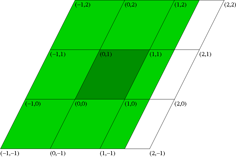
Wannier plot region in two dimensions. The parallelograms are different unit cells (or supercells). The dark green area corresponds to the definition (0:1,0:1). The complete (dark and light) green area corresponds to (-1:1.5,-1:2).
6.3.6. RESTART
If RESTART is set, Spex writes the Wannier functions (the U matrix) to the file “spex.uwan”
if it does not exist. Otherwise, the Wannier functions are read from “spex.uwan”. In the same way
the file “spex.kolap” is written or read containing the overlap of wavefunctions at neighboring
k points. These overlaps are needed for the maximalization procedure. (The file “spex.kolap” can be reused
if the orbitals in ORBITALS are changed but not the outer energy window, i.e., the first two
arguments.)
6.3.7. INTERPOL (WANNIER)
The keyword INTERPOL has already been discussed in Section 5.1.17. We explain it here for completeness and
provide further advice on its usage.
When given, Spex performs a Wannier interpolation for the reference mean-field system (output to the file “bands0”) and of the calculated GW (HF, COHSEX, et cetera) quasiparticle energies (output to the file “bands1”). It also gives, for each state, Wannier-function projections.
The quality of the Wannier interpolation depends crucially on whether the bands to be interpolated are representable in the set of
Wannier orbitals defined by ORBITALS. Finding the right parameters requires experience and often some experimentation. A good set of parameters (as
basis for further fine tuning) is usually found in the following way:
The bands to be interpolated should be predominantly described by some specific set of atomic orbitals, e.g., sp3 hybrids in diamond structure, t2g (eg) bands in octahedral coordination, or d bands crossed by itinerant s bands (perhaps including p bands) in transition metals. These orbital characters are provided in round or square brackets for individual atoms or atom types, respectively, see Section 6.3.1.
The lower band index is usually easy to determine
from the band structure (as it corresponds to the lowest band to be interpolated). In the case of an isolated group of bands
(i.e., with band gaps below and above), the upper band index should obviously correspond to the topmost band,
and a good interpolation is usually obtained with the ORBITALS definition and MAXIMIZE. Even just the first-guess orbitals
(obtained without MAXIMIZE) sometimes gives a good interpolation in this case.
However, in most cases, the bands to be interpolated do not form an isolated set of bands, and the band structure is entangled.
The upper (only in few cases also the lower) band index is then not uniquely defined. It is then recommended to simply set the
upper index as a wildcard (*) in the input file, which tells Spex to try to determine the index automatically. Often, the
automatic choice is already good enough. Usually, the Wannier interpolation of entangled bands requires
“maximally localized Wannier functions” that have been determined with a disentanglement procedure. So, we need
in addition the keywords MAXIMIZE and FROZEN. The parameter for the latter (upper bound for frozen window), when omitted,
will be determined automatically.
The keyword INTERPOL can be combined with PROJECT (Section 4.2.3) for the plot of “fat bands”.
As an example, we give the section WANNIER for an interpolation of the valence band structure of iron. The result is shown in
the figure above.
SECTION WANNIER
  ORBITALS 1 * (s,p,d)
  MAXIMIZE
  FROZEN
  INTERPOL
END
INTERPOL |
Perform Wannier interpolation of the input data (output “bands0”) and any calculated energies, e.g., GW (“bands1”).
The corresponding k-point path is defined by KPTPATH. |
INTERPOL "qpts" |
Same as before but the k-point path is taken from the file “qpts”. |
INTERPOL ENERGY "energy.inp" |
Same as INTERPOL but the energies for the interpolation written to “bands0” are taken from the file “energy.inp”.
The file format is identical to the one used for the global keyword ENERGY (Section 4.2.6). In most cases, the
resulting interpolation is identical to using INTERPOL together with the global ENERGY "energy.inp", but the
latter also reorders the eigenstates according to the energies, whereas the one-liner INTERPOL ENERGY "energy.inp" does not.
(Another obvious difference is that ENERGY changes the energies globally for the whole Spex run, while INTERPOL ENERGY
changes the energies only for the Wannier interpolation.) This reordering can affect the Wannier basis (if it is constructed in this
run) or would lead to an inconsistency with a Wannier U matrix read from “spex.uwan”. The latter case is caught by Spex,
which would then stop with an error (“inconsistent checksum”). All these problems are circumvented by the one-liner. |
INTERPOL "qpts" ENERGY "energy.inp" |
Combine the last two cases. |
6.3.8. BACKFOLD (WANNIER)
(*) The atoms of the basis of a Bravais lattice are not unique in the sense that one can
always translate an atom by an arbitrary lattice vector from r to r+R and still
describe the same periodic crystal with it. This means that any result (DFT, GW, …)
should be (and is) invariant with respect to such translations. However, there are exceptions
for methods that rely on a real-space representation. For example, the Wannier
interpolation (or its quality) does depend on the relative
positions of the atoms. (Other examples are the BSE Wannier approach, the GT method, and
off-site Hubbard U parameters.)
This is because it is based on a real-space cutoff of Hamiltonian matrix elements
\(\langle w^a_{\mathbf{R}n}|H|w^{a'}_{\mathbf{R}'n'}\rangle\),
where the two Wannier functions may be located at different atoms \(a\) and \(a'\).
(For clarity, we have included specific atom indices.) The cutoff criterion is with respect
to \(|\mathbf{R}-\mathbf{R}'|\). But the actual distance of the Wannier functions
is \(|\mathbf{r}_a+\mathbf{R}-\mathbf{r}_{a'}-\mathbf{R}'|\) with the atom positions
\(\mathbf{r}_a\) and \(\mathbf{r}_{a'}\) in the unit cell. So, the relative location
of the atoms (Wannier centers) do matter, and the interpolation works best when the atoms
are as close to each other as possible. Therefore, Spex automatically exploits the
translational freedom described above to shift the atoms so as to fulfill this condition as well as possible.
However, Spex might not find the optimal atomic configuration, or the user might want to
place the Wannier centers at certain atoms of his/her choice or avoid the atomic backfolding
altogether (see examples). For this purpose, there is the
keyword BACKFOLD, which expects as arguments one or more translation lattice vectors \(\mathbf{R}_a\),
maximally as many as the number of atoms. The Wannier centers will be placed at \(\mathbf{r}_a+\mathbf{R}_a\).
If there are less vectors than atoms in the unit cell, the remaining vectors are set to the null vector.
(Note for experts: The specific Wannier centers are taken into account in the construction of the Wigner-Seitz supercell
for Wannier interpolation in a procedure that is known as “use_ws_distance” in Wannier90. This procedure is always
activated in Spex but can be switched off in “wannier.f” by commenting out the macro “WS_wancent”.)
BACKFOLD (-1,-1,-1) (1,1,1) |
Shift first atom by \(\mathbf{R}_1=(-1,-1,-1)\) and the second atom by \(\mathbf{R}_2=(1,1,1)\). The other atoms (if any) are unshifted. |
BACKFOLD (0,0,0) |
Do not shift any atoms. |
6.3.9. IRREP (WANNIER)
(*) The set of Wannier functions should reflect the symmetry of the system. This can be used
to define matrix representations that determine how the Wannier functions transform when a
given symmetry operation is applied. These matrix representations can be used to speed
up the evaluation of certain Wannier-expanded quantities, for example, in spin-wave and
GT calculations. (The name IRREP is a bit misleading because the matrices are
not irreducible in general.) Unfortunately, Wannier90 tends to break the symmetry of the
Wannier set, so IRREP can, in most cases, not be applied to MLWFs. However, unless the
ORBITALS definition itself does not break the symmetry, the first-guess Wannier functions
reflect the full symmetry, and IRREP can be used.
6.3.10. UREAD (WANNIER)
(**) This keyword makes Spex read Wannier functions generated by Fleur. (Works only with old version of Fleur. Currently unmaintained.)
Note
Paragraphs discussing advanced options are preceded with (*), and the ones about obsolete, unmaintained, or experimental options are marked with (**). You can safely skip the paragraphs marked with (*) and (**) at first reading.